How to Send Out Google Classroom Enrollment Codes Using VLOOKUP and YAMM

In a previous blog, I had shown you how to Bulk create Google Classroom using Google Apps Script. In that blog, we created Google Classroom using the data from the Google Sheet using Google Apps Script. Further, into the blog, we wrote some code to paste the enrollment code into the Google Sheet.

Now that the classes have been created and the enrollment codes are ready, it’s time to send them to the students. Doing this manually will be a very hectic task. To reduce the work of the teacher, we are going to use the VLOOKUP Google Sheets formula and YAMM to send out the emails.

Step 1: Sample Google Sheet

The Google Sheet that we will be using in this blog contains the name and the email address of the students spread among different classes.

↗ Enlarge

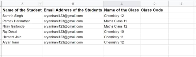
Entering the enrollment code for each student will take a long time, hence we are going to use the VLOOKUP formula in Google Sheets.

What is Google VLOOKUP in Sheets?

Google Sheets VLOOKUP function is short for Vertical Lookup. The function searches down the first column of a range for a key and returns the value of a specified cell in the row found. Let me show you how to use VLOOKUP in Google Sheets.

↗ Enlarge

This is the format for the VLOOKUP function, that contains the following parameters:

1. search_key = value to be searched
2. range = range for the search
3. index = column index of the value to be returned
4. [is_sorted] = indicated whether the specified column to search is sorted or not.

Using this formula we are going to specify the class that the student is assigned to, followed by the range to be searched and the enrollment codes column number and in the end, FALSE, since the range is not sorted.

Update: we have now published a full VLOOKUP guide.

Step 2: Apply the VLOOKUP Formula in Google Sheets

Now that the data is ready, it’s time to add the formula to the Google Sheet. To do that follow these steps:

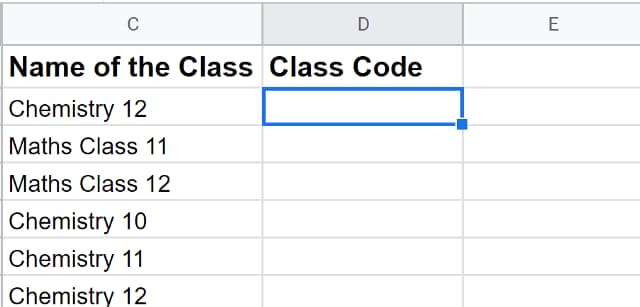
1. Select the cell where you want to apply the formula

   ↗ Enlarge

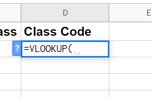
2. To apply the formula start by typing VLOOKUP( that will bring up the formula.

   ↗ Enlarge

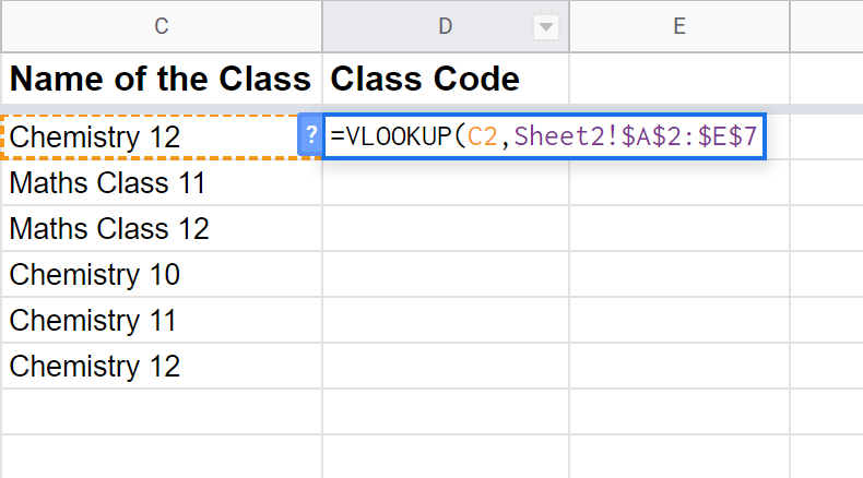
3. The first parameter that we pass in the formula is the name of the class. This is the value that will be searched in the sheet.

   ↗ Enlarge

   VLOOKUP(C2,Sheet2!$A$2:$E$7
   

   Copy code

4. Next we have to pass the range (Sheet2!$A$2:$E$7) in the formula. We are getting data from the second sheet, so first comes the name of the sheet followed by the range that needs to be searched through. In the range specified, we have added a dollar sign, which is known as absolute cell reference. Absolute cell reference will keep the row/column constant in the formula.

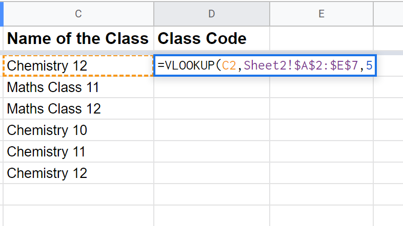
5. Next we have to pass the column number from which the value has to be returned. Since my enrollment codes are stored in column E, in the previous Google Sheet, I am going to be passing column number 5 as the third parameter in the VLOOKUP formula.

   ↗ Enlarge

6. After the column number, we are going to type in FALSE since our data is not sorted.

   ↗ Enlarge

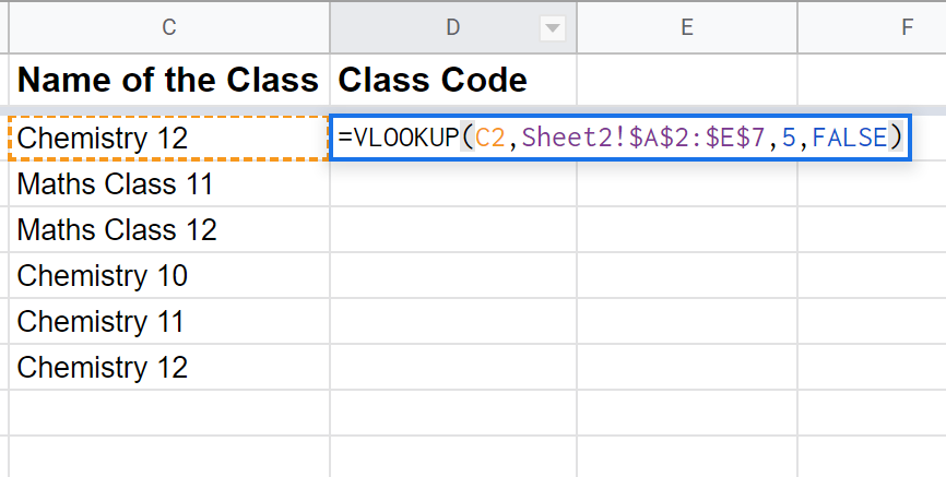
On clicking enter, you will see that the Enrollment code for the given class has been as shown below.

↗ Enlarge

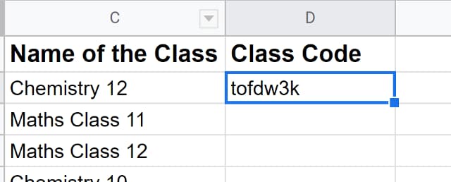
To apply the formula to all the cells below just click on the blue box and drag it down. We can do this thanks to the absolute cell reference. Even if we drag the formula till the end of the sheet, the range in the formula will stay constant, due to the $ we added to the range.

↗ Enlarge

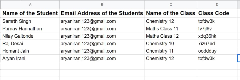
Here you can see all the enrollment codes have been imported into the sheet.

Step 3: Send out the Enrollment Codes

Now that we have got all the codes in the Google Sheet, it’s time to send the emails out using YAMM.

What is YAMM?

YAMM(Yet Another Mail Merge) is an easy to use Mail merge where you select a draft created in Gmail and replace all the variables from a Google Sheet. It will send automatic personalized emails to the contacts specified in the spreadsheet.

Step 4: Install the Yet Another Mail Merge Add-on

Before we get into creating the draft for the email, we have to install the YAMM add-on to our Google Sheet. I have covered these steps in my previous blogs, read how to send bulk emails using YAMM to know more.

Step 5: Create your Google Classroom Email Format

To create the draft, you have to follow the same steps that you follow to write an email. To create your draft, follow these steps:

1. Go to gmail.com

2. Click on Compose and start writing your email draft.

3. We have to replace the variables in the draft with the data in the Google Sheet. To do that you need to specify the column names that you want to replace in the draft like this.

   ↗ Enlarge

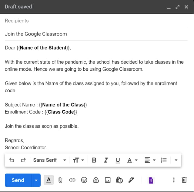
   Dear {{Name of the Student}},
   
   With the current state of the pandemic, the school has decided to take classes in the online mode. Hence we are going to be using Google Classroom.
   
   Given below is the Name of the class assigned to you, followed by the enrollment code
   
   Subject Name : {{Name of the Class}}
   Enrollment Code : {{Class Code}}
   
   Join the class as soon as possible.
   
   Regards,
   School Coordinator.
   

   Copy code

4. Here I have done the following:

   • Here I wanted to put the name of the student at the beginning of the email, so I put in the column name where the names are stored.
   • The same is for all the other variables that I have called in the email draft.

5. After you are done creating the draft, save and close the draft.

Step 6: Send the Emails

Now that we have installed the YAMM Add-on, created the email draft, it’s time to send out the emails. To send out the emails, follow these steps:

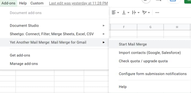
1. Go to Add-ons and click on Yet Another Mail Merge and start the mail merge.

   ↗ Enlarge

2. On clicking Start Mail Merge, it will bring up a box where you need to put in some details.

   Here you need to specify the sender name, followed by the email template that you want to use.

   ↗ Enlarge

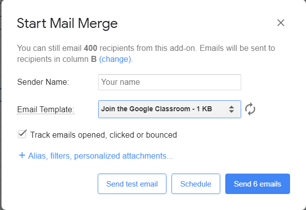
Now that we have added all the features that we need, let’s send out the emails. You have the following options:

1. Send all the emails
2. Schedule the emails
3. Send a test email to check whether everything works fine.

For now, we are going to go ahead and send the emails by clicking on Send 10 Emails.

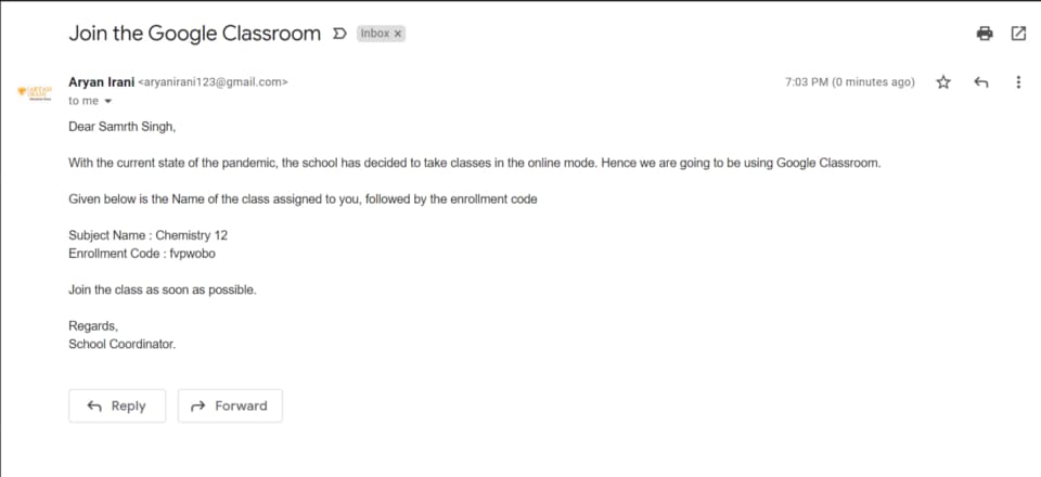
Step 7: Check the Emails

Here you can see on successful execution the emails have been sent and all the details have come in properly.

↗ Enlarge

Summarizing how to do VLOOKUP in Google Sheets to send Google Classroom Enrollment Codes

In this blog, we saw how to send out bulk emails using YAMM. We started out by using the Google Sheet VLOOKUP formula to get the enrollment codes from one sheet to another. Next, we installed the YAMM Add-on followed by adding some settings and then sent the emails. I hope you have understood how to send you the Enrollment Codes using YAMM.